An Introduction to NCBI Cloud Computing for Virologists

Workshop Description: As DNA sequencing becomes a commonplace tool in biological research, the need for accessible, scalable, and secure computational environments to process this deluge of data is growing. NCBI has partnered with leading cloud computing providers to provide tools and data to this growing industry. This workshop is designed for experimental virologists without cloud computing experience. While not required, it is most useful for researchers who do sequence-based research and who have some familiarity interacting with a Linux command-line.
In this online, interactive workshop you will learn how to:
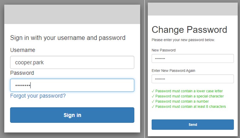
1) Navigate to https://codeathon.ncbi.nlm.nih.gov and login using the following credentials:
Username: Email prefix (everything before the @ in your email address) For example, if your email address is example@gmail.com, then your username will be example
Password: See the Workshop Zoom Chat for today’s password. You will be prompted to create a new permanent password after your first login.
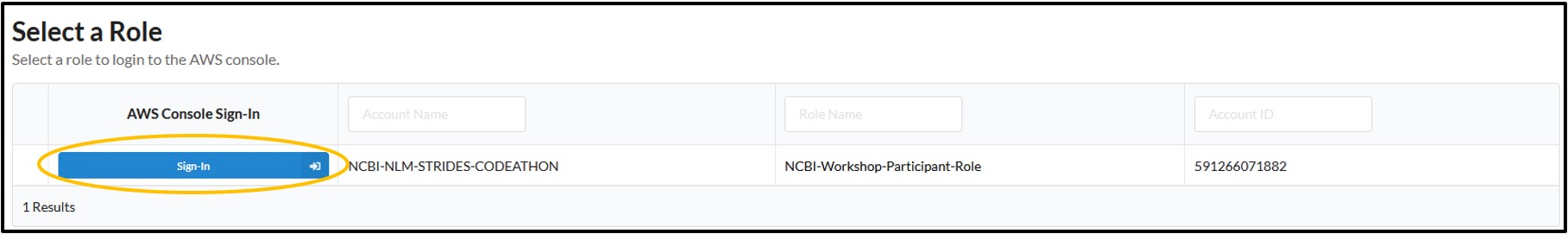
2) Click Sign-In under the AWS Console Sign-In column on the new page
NOTE: If you are prompted to explore the “New AWS Console Home”, click Switch to the new Console Home, we want the latest and greatest!
3) If you see AWS Management Console like the screenshot below, you have successfully logged in to the AWS Console!
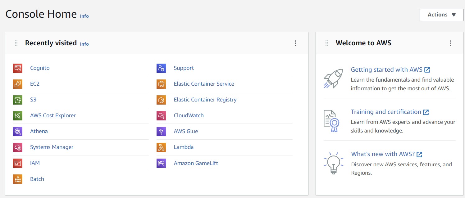
NOTE: If you are logged out or get kicked out of the console, simply return to https://codeathon.ncbi.nlm.nih.gov and log in again (remember your newly created password!) to get back to the console home page.
NOTE: This login method is unique to the workshop. If you want to create your own account after the workshop, visit the link below and follow the steps: https://aws.amazon.com/premiumsupport/knowledge-center/create-and-activate-aws-account/
Before we can properly use the cloud we need to make an S3 bucket that can save our data from each tool. So, let’s go make one!
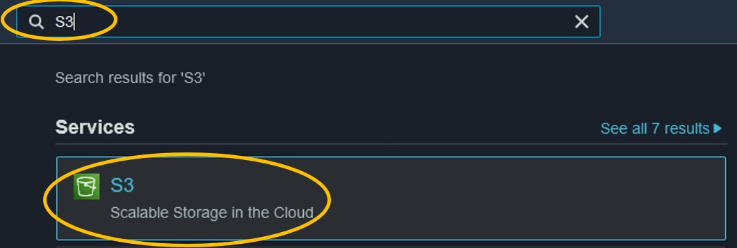
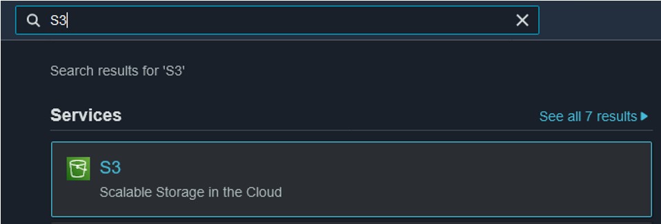
1) Use the search bar at the top of the console page to search for S3 and click on the first result
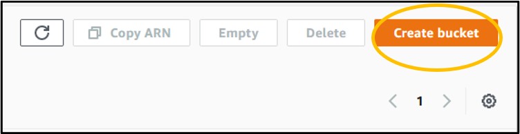
2) Click the orange Create Bucket button on the right-hand side of the screen
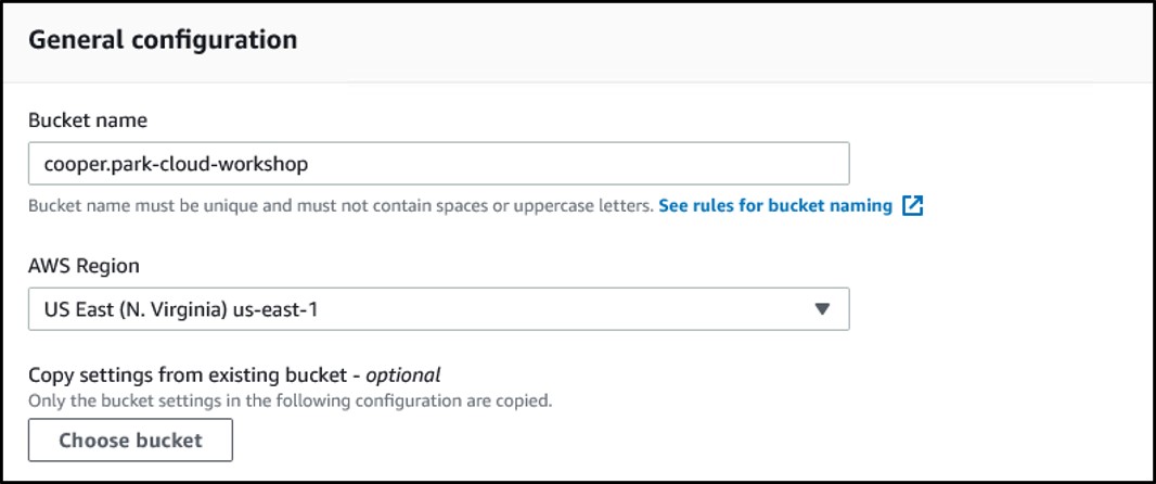
3) Enter a bucket name and make sure the region is set to US East (N. Virginia) us-east-1
S3 bucket names must be completely unique.
For this workshop, use the format <username>-cloud-workshop where <username> is the username you used to login
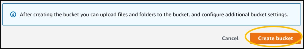
4) Ignore the rest of the settings and scroll to the bottom of the page. Click the orange Create Bucket button.
5) Clicking the button will redirect you back to the main S3 page. You should be able to find your new bucket in the list. If so, you have successfully created an S3 bucket!

Now that we have an S3 bucket ready, we can go see what the Athena page looks like!
One of the most common uses of the cloud is simply renting some computer space from the cloud provider to run some code and generate data. Today, we’ll setup an EC2 instance to generate and align a viral consensus sequence with it.
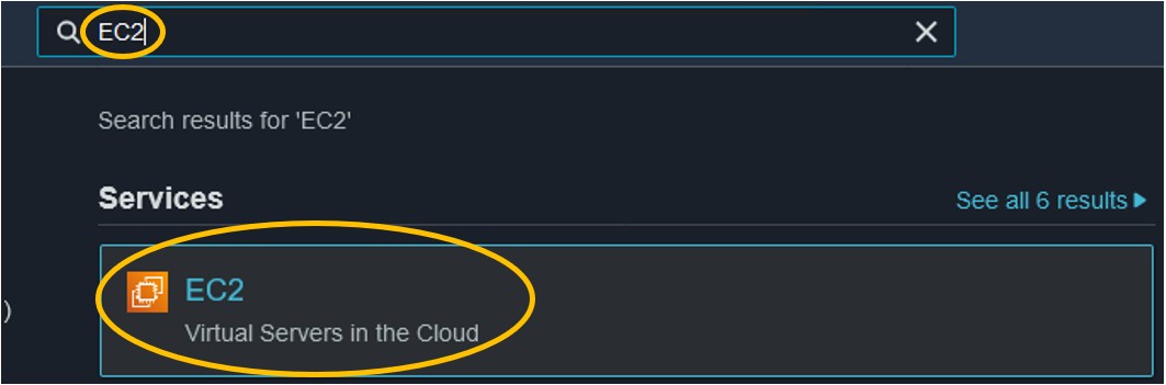
1.1) Use the search ar at the top of the console page to search for EC2 and click on the first result
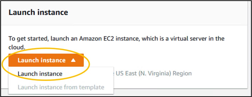
1.2) Scroll down a little and click the orange Launch Instance button and Launch Instance from its drop-down menu
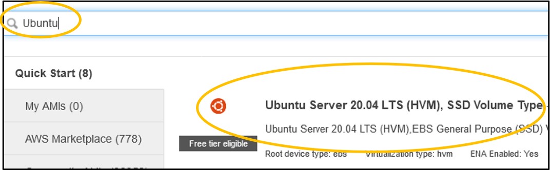
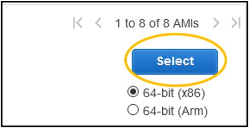
1.3) On the Step 1: Choose an Amazon Machine Image (AMI) page - type Ubuntu into the search bar and hit enter (top image) then click the blue Select on the right hand-side of the Ubuntu Server 20.04 image option (bottom image).
1.4) On the Step 2: Choose an Instance Type page - use the filter menus near the top of the menu to set the Instance Family to m6i
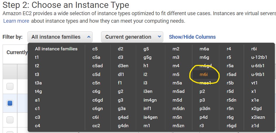
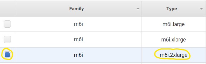
1.5) Look to the table below the filter buttons and check the box in the 2nd row from the top where the type is m6i.2xlarge
1.6) Click Next: Configure Instance Details

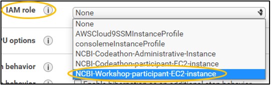
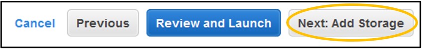
1.7) On page Step 3: Configure Instance Details - set the IAM role to NCBI-Workshop-participant-EC2-instance (top image). Leave all other settings alone and click Next: Add Storage in the bottom right (bottom image)
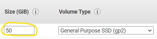
1.8) On page Step 4: Add Storage - Change the Size (GiB) to 50 (top image), then click Next: Add Tags in the bottom right (bottom image)

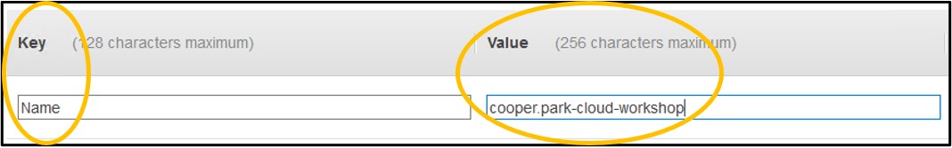
1.9) On page Step 5: Add Tags - Click Add Tag on the left side of the screen (top image). In the new row set the Key to be Name and the Value to be <username>-cloud-workshop just like we did with the S3 bucket earlier (bottom image). Remember, <username> is the username you logged into the console with.

1.10) Click Next: Configure Security Group in the bottom right of the screen

1.11) On page Step 6: Configure Security Group - Near the top of the screen, click Select an existing security group. Then click the box of the Default row at the top.
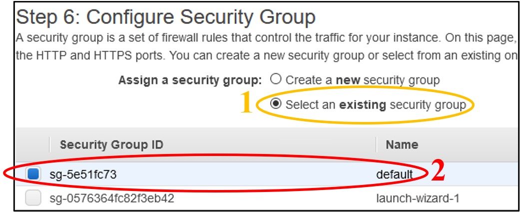
NOTE: This “default” network setting configuration leaves the instance open to public access. Typically you will want to restrict this to only trusted IP addresses, but for the purposes of the workshop we keep this open so there is no need to troubleshoot network issues. To balance this security flaw, we will restrict access to our instances with another instance feature in a few more steps.
1.12) Click Review and Launch in the bottom right of the screen

1.13) On page Step 7: Review and Launch – You should see two warnings at the top of the screen denoted by the symbol below. You can disregard these.
NOTE: The first warning tells us that our instance configuration will cost us money. The second warning tells us that our network settings make our instance publicly accessible, which is discussed in the above “NOTE”.

1.14) Click Launch in the bottom right of the screen.

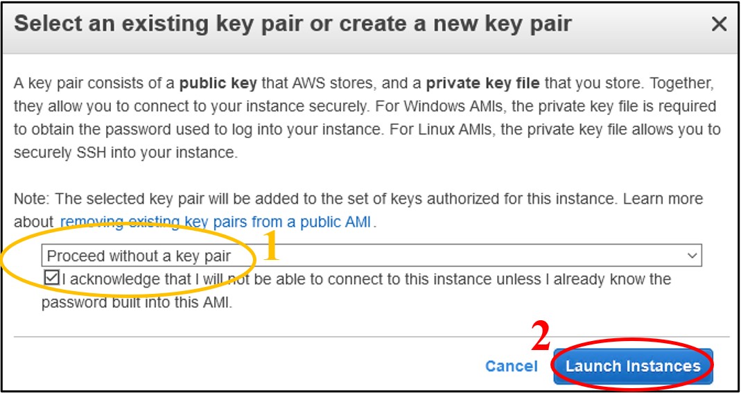
1.15) On the pop-up menu – change the first dropdown menu to Proceed without a key pair and check the box below it to acknowledge the change. Finally, click Launch Instances in the bottom right of the popup.
NOTE: Key pairs are used to access an instance outside of the AWS console, like through SSH. We won’t be using these other methods so we can skip the key pairs here without affecting our ability to do the workshop. Additionally, by disabling the key pairs we also prevent external access to the instance. (This is how we will secure our instances for the workshop)
1.16) On the Launch Status page – Click View Instances in the bottom right

1.17) On the Instances page – Find your instance in the table of created instances and look to the Status Check column to see the status of yours.

1.18) Refresh the page occasionally until the Status Check column changes to 2/2 checks passed for your instance. This means we can now log into the instance.
NOTE: There are several states this column can have.
2/2 checks passedis the final status. So, if you see anything else in the Status Check column, the instance is not ready to go.

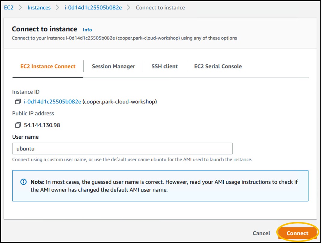
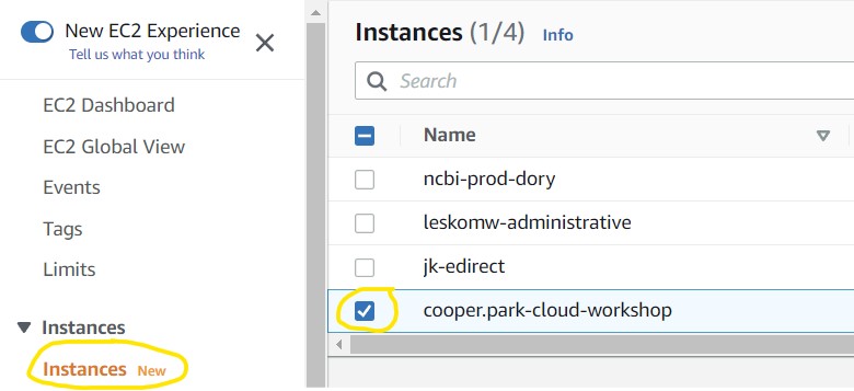
1.19) Check the box to the left of your instance name (top image) to select the instance, then click Connect in the top right to head to the instance launcher (bottom image)


1.20) On the launcher page, click Connect in the bottom right. This will launch a new tab in your browser and connect you to your remote computer!
Before we can do our analyses, we need to install the required software into our the instance. There are many programs necessary to make today’s exercise work. So rather than typing all of that code out ourselves I have prepared a script that we will use to install the programs for us.
1.21) First we need to download the script I have written for this workshop. Click the copy button on the code block below and paste it into your terminal
wget https://raw.githubusercontent.com/parkcoj/Intro-to-NCBI-Cloud-Computing-Virologists/master/workshop_materials/EC2_workshop_installations.sh
1.22) Next, we need to tell our computer that this new file is a script we want to run. The following code block will give our computer permission to run the script, and then run it.
chmod +x EC2_workshop_installations.sh && nohup ./EC2_workshop_installations.sh
WARNING: This script can take up to 15 minutes to run due to the number of programs being installed. It’s likely that your connection to the computer will time-out during then and you will be forced to reconnect. DON’T WORRY! The
nohupcommand we added above will ensure that the installation continues even if you get disconnected.
1.23) Now that all of our programs are installed we need to configure the computer to access these programs with some shortcuts. The following command will create those shortcuts in our computer so it is easier to run the new programs.
echo "export PATH=$PATH:$PWD/hisat2-2.2.1:$PWD/sratoolkit.2.11.2-ubuntu64/bin" >> .bashrc && source ~/.bashrc
1.24) Finally, although the installation script included the SRA Toolkit, we still need to configure it to start working. The following steps will configure the SRA Toolkit
vdb-config -i
The page that opens is an interactive graphic display where we can customize the settings necessary for SRA toolkit to run. For today we only need to change one setting, so here are the buttons to hit to do that.
A to change to the AWS tabR to enable reporting of your cloud identity (telling NCBI that you sent the command from an AWS computer)S to save the changesX to close the interactive browserWe can (finally) do the analysis we want! Like the installation process, there are a lot of steps in the analysis that each take different lengths of time to complete. To simplify and optimize this process we are going to download a second script online that does the process for us. We will walk through the steps soon, but remember that they all happen in the same script.
1.25) To download the script, run the following command:
wget https://raw.githubusercontent.com/parkcoj/Intro-to-NCBI-Cloud-Computing-Virologists/master/workshop_materials/SRA_to_consensus.sh
1.26) Next, let’s tell the computer it’s okay to run the script…
chmod +x SRA_to_consensus.sh
1.27) And finally, we run the script! I have designed the script to require us as a user to provide the SRA accession we want to build a consensus from. So the following command will run the script with our case study accession SRR15943386
nohup ./SRA_to_consensus.sh SRR15943386
We use the nohup command on this script also, because it can take up to 1 hour to run! So we will let this program do its thing for a bit while we go do some other exercises. Let’s navigate back to our AWS console tab and move on to some other work.
You can also use the SRA Run Selector on the NCBI website to download data from NCBI directly to your S3 bucket! Find more information and a tutorial here:
https://www.ncbi.nlm.nih.gov/sra/docs/data-delivery/
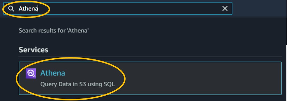
2.1) Use the search bar at the top of the console page to search for Athena and click on the first result
2.2) If you are prompted to visit the new Athena console experience, do it. We want to use the latest and greatest!

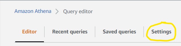
2.3) To make sure Athena saves our search results in the correct S3 bucket, we need to tell it which one to use. Good thing we just made one, eh? Click Settings in the top left of the screen
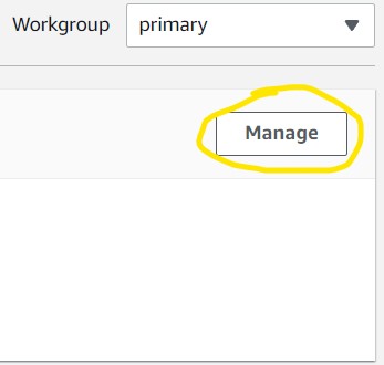
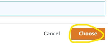
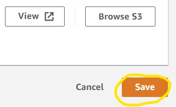
2.4) Click the Manage button on the right (1st image) then Browse S3 on the next page (2nd image) to see the list of S3 buckets in our account. Scroll to find your S3 bucket then click the radio button to the left of the name and click Choose in the bottom right (3rd image). Finally, click Save (4th image).

Now that we can save Athena results we can run some searches! The very last step to doing that is to import the table we want to search into Athena using another AWS service - Glue. However, to save time, this has already been done prior to the workshop by the instructor.
For the detailed instructions on using AWS Glue to add a table to Athena, visit the Supplementary Text: Instructions for AWS Glue!
These steps aren’t necessary to do before every Athena query, but they are useful when exploring a new table.
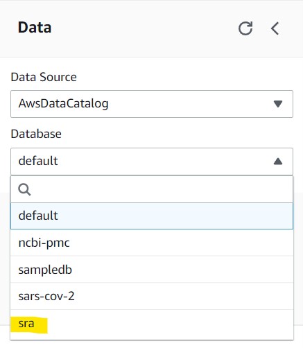
2.5) Navigate back to the Editor tab and click the dropdown menu underneath the Database section and click sra to set it as the active database. If you do not see this as an option, refresh the page and check again.
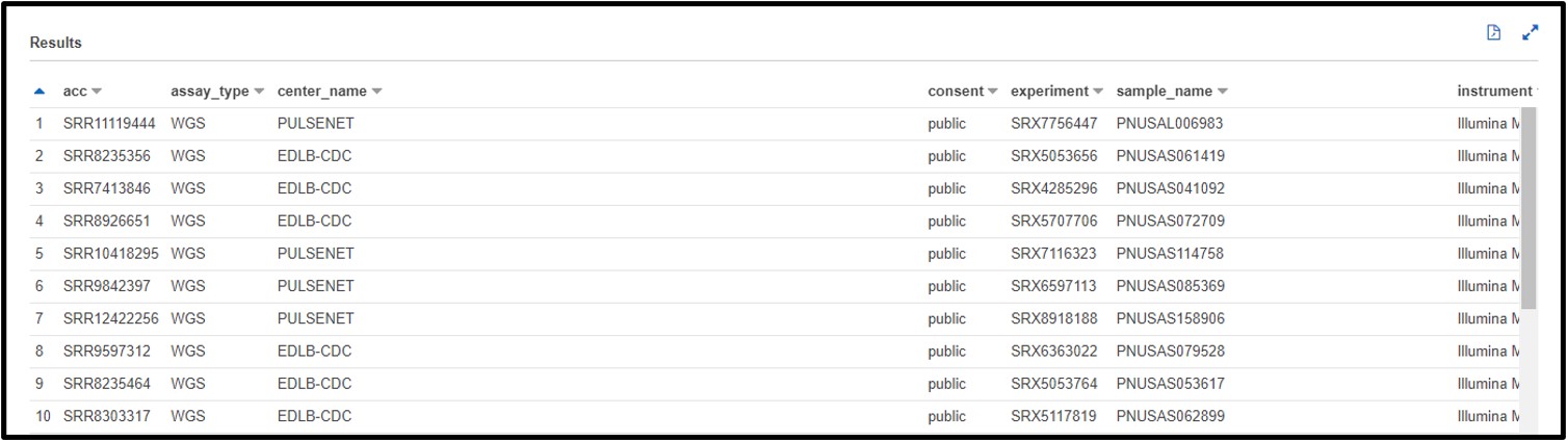
2.6) Look at the Tables section and click the ellipses next to the metadata table, then click Preview Table to automatically run a sample command which will give you 10 random lines from the table
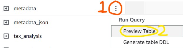
You can also click the + button next to the Metadata name to see a list of all the columns in the table.
For SRA based tables, you can also visit the following link to get the definition of each column in the table: https://www.ncbi.nlm.nih.gov/sra/docs/sra-cloud-based-examples/
Obviously we already know what accession we need for the analysis, but what else can we learn about our sequence?
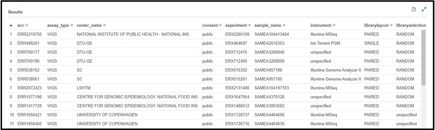
2.7) Now the accession we gave to our consensus sequence analysis was SRR15943386, but we don’t know exactly which column that is associated with. So, scroll through the preview table we made earlier to find a column filled with similar values.
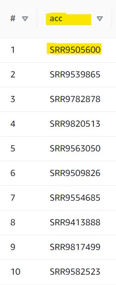
The Preview Table query we used to make this example pulls random lines from the table, so the values within your table may look different from this screenshot. The important info for us is that each value in this acc column starts with “SRR” (or “ERR” or “DRR”)
2.8) Now that we know which column to query for our data (acc), we can build the Athena query. Look to the panel where we enter our Athena queries. Click New Query 1 to navigate back to the empty panel so we can write our own query.
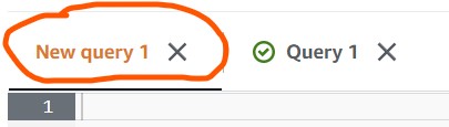
Fun fact: If you navigate back to Query 1 you should still see the result table for that query! Athena will save that view for you until you run a new query in that tab or close the webpage.
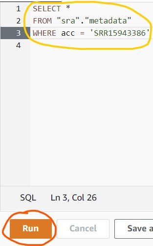
2.9) Copy/paste the following command into the query box in Athena (circled in yellow), then click the blue Run Query button (circled in red).
SELECT *
FROM "sra"."metadata"
WHERE acc = 'SRR15943386'
2.10) If you see a results table with one row like the partial screenshot below, you have successfully found your data!
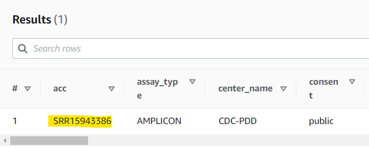
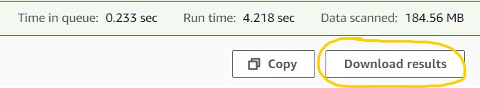
2.11) Click the Download results button on the top-right corner of the results panel to download your file to your computer in CSV format. You should be able to open this in Microsoft Excel, Google Sheets, or a regular text editor (e.g., Notepad for PC, TextEdit for Mac).
Want to challenge yourself? Visit the supplementary text (section: SQL challenges) to find some questions you can build your own SQL query for. Plus, find more advanced SQL query techniques and a deeper breakdown of the SRA metadata table too!
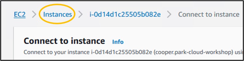
3.1) Let’s navigate back to the EC2 instance we made in Objective 1 and see our progress. If you kept your original EC2 instance tab open, you can simply refresh the tab to reconnect to it, otherwise you can reconnect using the Instances table on the EC2 console page
To know if the script has finished, we need to check two things.
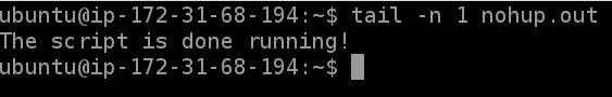
The script itself is designed to tell us when it is complete. In the log file nohup.out there should be a line that says "The script is done running! I hope this worked!". We can look for this line to check if the script is complete.
3.2) Run the following command to pull the last line from the log file and see if our program completed:
tail -n 1 nohup.out
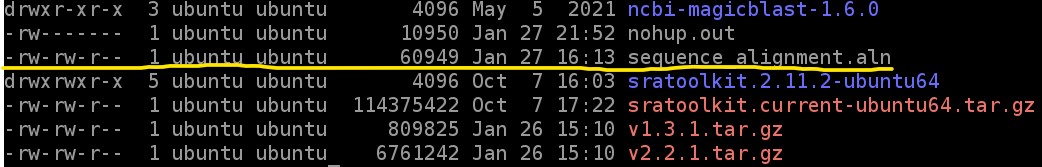
3.3) Next, to see if our alignment file was created, type
ls -l
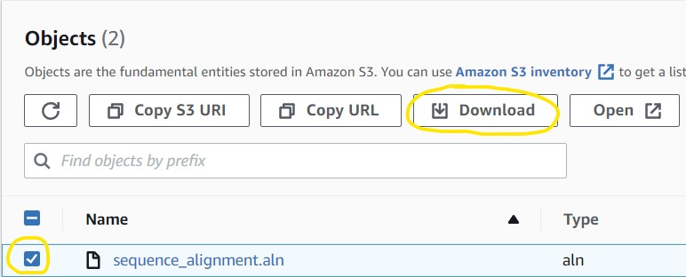
to get a list of files on the EC2 instance. Look through that list for sequence_alignment.aln to know if we got the final file we want (the screenshot below is truncated, you will have more files)
If the file is present, then our work is done! We just need to move those results to our S3 bucket so we can access the data outside of our EC2 instance. Run the following AWS CLI command to copy the files to your S3 bucket.
REMEMBER: You will need to replace the
<username>piece of the command with your own login username to make it match your S3 bucket name. So copy/paste the command into your terminal, then use the arrow keys to move your cursor back through the string and change the name to your own bucket.
aws s3 cp sequence_alignment.aln s3://<username>-cloud-workshop
3.4) We should now be done with our remote computer (aka: EC2 instance). Go ahead and close the browser tab your instance is open in.
3.5) In the console webpage, click the blue Instances button at the top of the instance launcher page
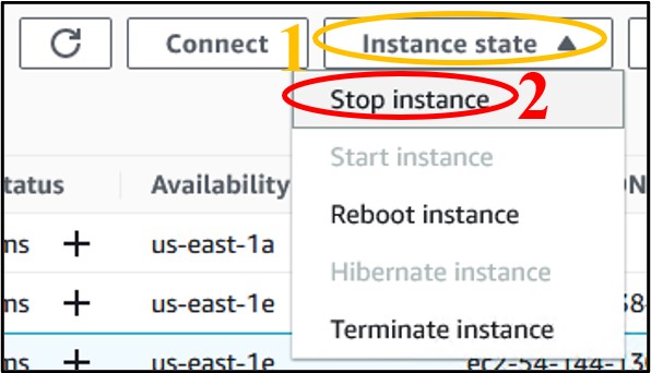
3.6) We don’t want to leave an instance on while not using it, because it costs money to keep it running. So, let’s shut it down, but not delete it, just in case we want to use it later. Check the box next to your instance (top image) then click the Instance State drop-down menu and select Stop Instance (bottom image).

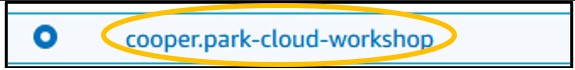
3.7) Finally, we need to check on the file in our S3 bucket and download it for use in our final Objective. Navigate back to the S3 page (use the search bar at the top of the console page) (top image) and click on your bucket name (bottom image) to see its contents
3.8) You should see the file in your S3 bucket. Simply click on the checkbox next to the filename and select Download from the list of options at the top of the page
4.1) Open a new tab in your web browser and go to https://www.ncbi.nlm.nih.gov/projects/sviewer/
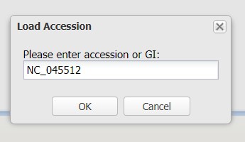
4.2) Click enter an accession or gi to choose the reference sequence. We aligned our sequence against the NCBI RefSeq record NC_045512, so enter the accession NC_045512 into the box provided and click OK
The Sequence Viewer page comes pre-loaded with several tracks aligned against the chromosome. Most of these are not useful to us today, so let’s configure the page to be a bit easier to read.
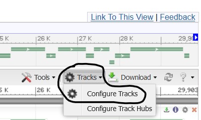
4.3) Click the Tracks button in the top-right corner of the viewer page and select Configure Tracks
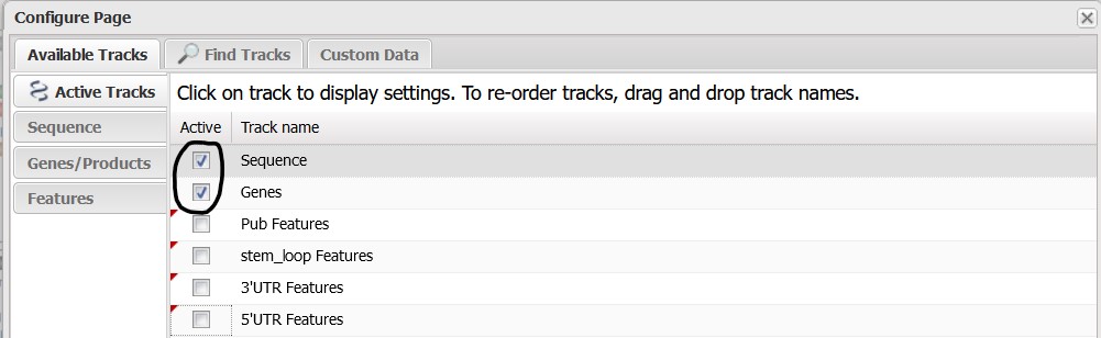
4.4) Deselect all of the tracks on this page except Sequence & Genes to remove those tracks from the Sequence Viewer panel.
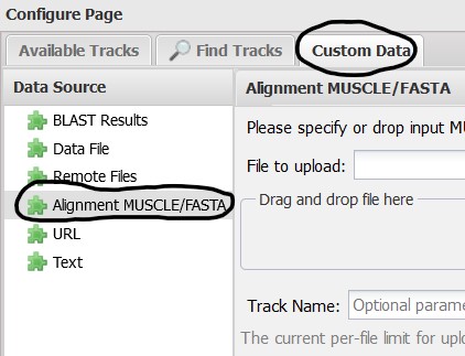
4.5) While we’re at it, lets add our own data track, select the Custom Data tab at the top of the pop-up menu. We created a sequence alignment so select the Alignment MUSCLE/FASTA Data Source from the menu on the left of the new page.
4.6) Next, find the file we downloaded from our S3 bucket and drag-and-drop it onto the upload box. You can also use the Browse button if that is more convenient for you. You should also provide a name for the track so it is easy to identify in the Sequence Viewer. Here I use SRR15943386 Alignment. Click Upload to add the track to the Sequence Viewer
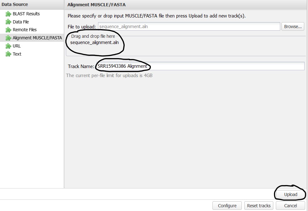
4.7) Click Configure to see the track on your Sequence Viewer
NOTE: When the track is first uploaded you may see a long red bar. This is a graphical bug. It will resolve itself as we continue with the exercise
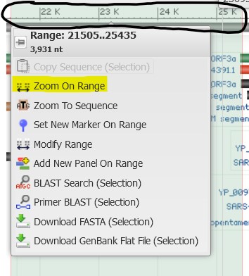
4.8) The mutation we are looking for is found in the S protein. Click-and-drag your mouse across the coordinate plot at the top of the Sequence Viewer to outline the region of the genome where the S protein is located (it does not have to be exact). Select Zoom on Range from the pop-up menu to refocus the viewer on that highlighted region.
The alignment track shows each point of variation between the RefSeq Sars-CoV-2 sequence and our own sequence. Below are a few of the common variations:
We can see within the S protein that there are several points of variation as indicated by the several vertical red bars interspersed within the gray alignment bar. Our variation of interest in this protein is N501Y which, in plain text, means “the 501st amino acid in the S protein was an Asparagine (N), but is now a Tyrosine (Y)”. To convert this name into nucleotide coordinates we can do some basic math.
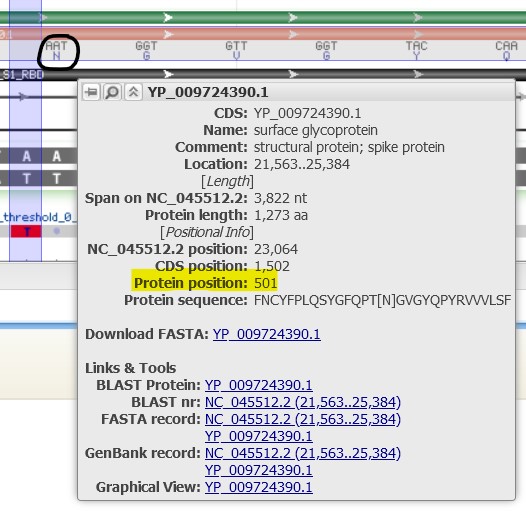
4.9) Hover your mouse over the S protein Gene bar (the green one). Find the location information to note where the start/stop coordinates are for the gene within the genome.
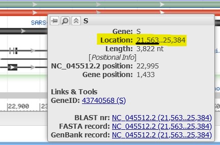
If the start position of the gene is 21,563 and we want to look 500 amino acids into the protein, then the following equation should give us the correct genomic coordinate to jump to:
21563 + (500 * 3)
which gives us 23,063 bases. Let’s use this to jump to the correct position in the gene.
4.10) In the search bar at the top-left of the screen type 23,063 and hit enter to quickly focus the Sequence Viewer on our desired location
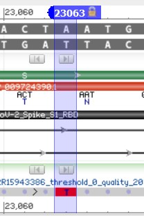
4.11) Look, a mutation! We can hover over the N amino acid to confirm that this is indeed the 501st amino acid.
4.12) Our sequence shows a codon mutation from AAT to TAT. Use the codon table below to find the new Amino Acid coded for by our sequence:
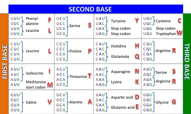
4.13) It looks like we have indeed spotted a N501Y mutation in our sequence. Well done! You can see how visualizing this alignment allowed us to rapidly identify points of variation between our strain and the Wuhan one, but we took it a step further to investigate a specific variant as well to confirm that it matched our expectations.
This concludes our exercise on navigating the AWS Cloud computing console and several of its most popular cloud services. We hope that you are motivated to take these skills and tools with you and explore how they can benefit your own research. You can find links to many useful resources to help you below.
The examples you have done today are a very small glimpse into how you can move your traditional research into the cloud. Unfortunately, 3 hours is hardly enough time to demonstrate the power of the cloud and how it can improve your workflows! So how can the cloud improve what we did today? Here are some examples that you can think about for this case study:
AWS
Sequence Viewer
SRA
3rd Party Tools
In order search through a table (like the SRA metadata table) you need to load it into Athena. If this is your first-time accessing Athena, you won’t have any data tables loaded! Therefore, your first step should be to add a table to Athena. There are three ways you can add a table to Athena:
Create the table using SQL commands (we are not SQL experts here…yet, so we won’t do it this way)
Add the table manually from an S3 bucket (although the SRA metadata is stored in its own S3 bucket, we don’t know the format of the table, so we can’t do it this way)
Use another AWS service called AWS Glue to automatically parse a table and load it into Athena for us using a “Crawler” (this is what we will do)
Note: Although AWS Glue is the most convenient method, it is also the only one to cost money. To parse the SRA metadata table it will be… ~$0.01.
This section will walk through the steps taken during the AWS Glue demo to prepare the SRA metadata table for Athena queries.
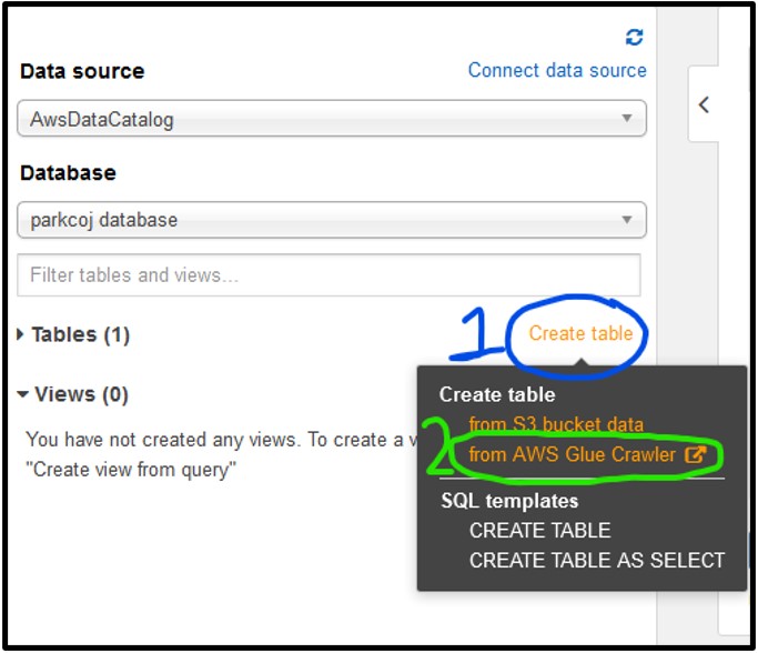
1) To start working with AWS Glue, navigate to the Tables section of the Athena page on the left-hand side, then click Create Table and select from AWS Glue Crawler as seen below. If you see a pop-up about the crawler, just click Continue.
2) The settings for this crawler should e set as described below:
Next page
Next page
Next page
Next page
Next page
Next page
Next Page
Click Finish
3) You should now be on the Crawler page for AWS Glue. Here you can manage and run crawlers. Click the checkbox next to the new crawler and select Run Crawler
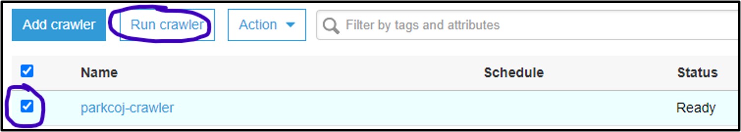
4) If it worked, you should see the Status column say Ready again, and the Tables added column should have changed to 1:

5) The table should now appear in Athena and you can follow the same steps described in section Exploring Athena Tables above.
Now that you have a handle on how SQL commands work, let’s try some examples! Remember, you can use the “Tables” section on the left-hand side of the page to find out which columns you can filter by in your table.
If you find yourself stumped on the answer to any of these, or just want to check your answer, click the dropdown box underneath the question to reveal the solution and see a screenshot of the results table!
a) You just came across a new paper with lots of great sequence data. You want to add that data to your own research so you jump to the paper’s Data Availability section (because all great computational papers have one!) and see that the data was stored in an SRA study under the accession SRP291000. Write a SQL command in the query terminal to find all data associated with the SRA study accession SRP291000:
SELECT * FROM "sra"."metadata" WHERE sra_study = 'SRP291000'
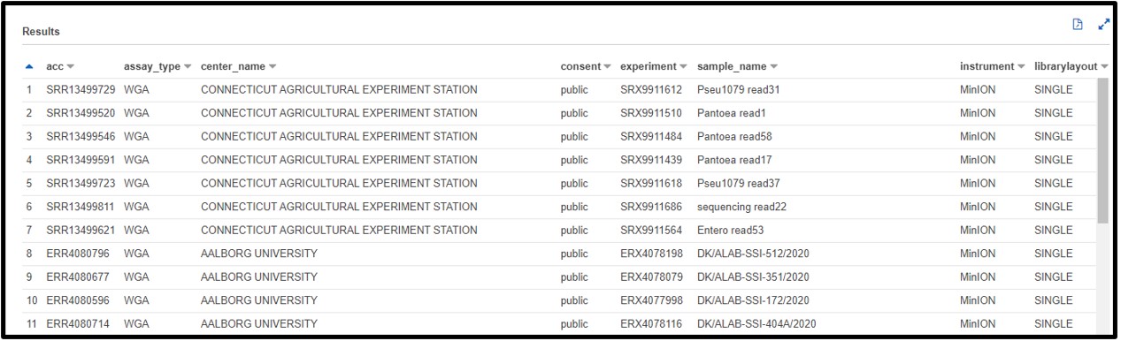
b) You are working on a new genome assembly tool for short-read sequences. However, you don’t have any reads of your own to test it! You know that SRA metadata includes the sequencing platform reads were generated on, so you decide you want to check there. Write a SQL command in the query terminal to find all data sequenced with the OXFORD_NANOPORE platform.
SELECT * FROM "sra"."metadata" WHERE platform = 'OXFORD_NANOPORE'
Now let’s get a little bit more complicated with our queries by combining multiple filtering conditions together. For example, see the command below:
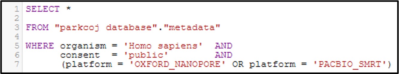
In this command we use the AND statement to add multiple requirements for our data. Specifically, we added a second criteria where the consent = public (aka: The data is not under restricted access). Additionally, we add a more complex requirement by using an OR statement for the platform column to ask for data that was generated by the OXFORD_NANOPORE OR PACBIO_SMRT sequencing platforms. Overall, by running this command we will only get the data that fits all 3 conditions.
Note: Make sure you include parenthesis around an OR statement as seen above, otherwise the query may not work as intended.
Here’s a few brain teasers to flex your new SQL skills! Remember, if you are stuck you can click the dropdown box underneath the question to reveal the solution and see a screenshot of the results table!
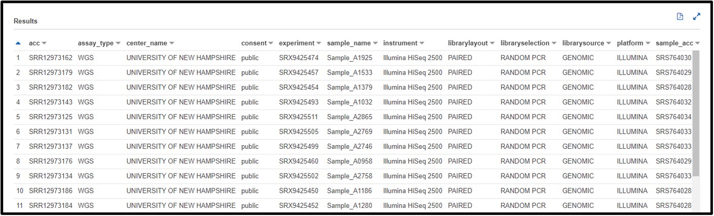
a) After testing your genome assembly tool from earlier, you realize that not all Illumina datasets are created equally! It turns out you only need WGS (Whole Genome Sequencing) genomic data to properly validate your software. Also, you noticed that there was some metagenomic and transcriptomic data mixed in with your test cases. So, this time you are just going to look for “genomic” datasets. Write a SQL command in the query terminal to find all WGS assay_type data sequenced on the ILLUMINA platform and a GENOMIC library_source.
SELECT * FROM "sra"."metadata" WHERE platform = 'ILLUMINA' AND assay_type = 'WGS' AND librarysource = 'GENOMIC'
b) You are designing a population-level epidemiological survey of some bacterial pathogens from samples collected across Europe. You decide you want to get some preliminary data on Escherichia coli (or maybe Staphylococcus aureus…) from the SRA, but you aren’t picky about what kind of sequencing is done just yet. Write a SQL command in the query terminal to find all sequences collected from the continent Europe and are from the organism Escherichia coli or Staphylococcus aureus.
Hint: The column header for the continent is not very intuitive. Try using the “Preview Table” option from the “Tables” tab described earlier to find a column that would fit.
SELECT * FROM "sra"."metadata" WHERE (organism = 'Escherichia coli' OR organism = 'Staphylococcus aureus') AND geo_loc_name_country_continent_calc = 'Europe'