An Introduction to NCBI Cloud Computing for Biologists

Workshop Description: As DNA sequencing becomes a commonplace tool in biological research, the need for accessible, scalable, and secure computational environments to process this deluge of data is growing. NCBI has partnered with leading cloud computing providers to provide tools and data to this growing industry. This workshop is designed for experimental biologists without cloud computing experience. While not required, it is most useful for researchers who do sequence-based research and who have some familiarity interacting with a Linux command-line.
In this online, interactive workshop you will learn how to:
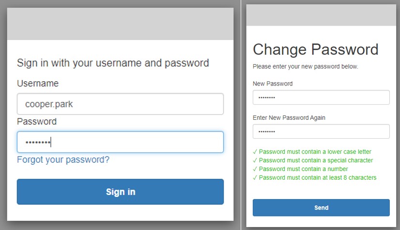
1) Navigate to https://codeathon.ncbi.nlm.nih.gov and login using the credentials below (left image) and create a new password after logging in (right image)
Login: Email prefix (everything before the ‘@’ in your email address, all lowercase)
Password: Watch the zoom chat for the password!
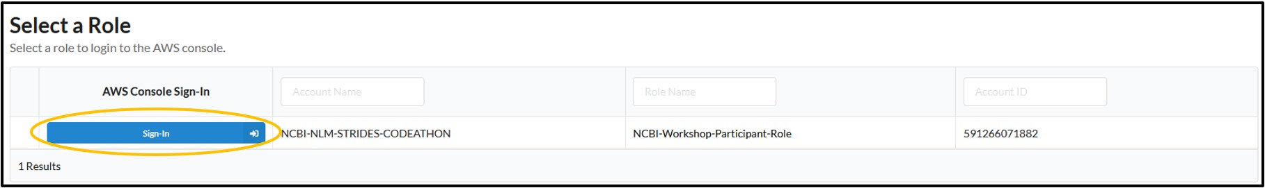
2) Click Sign-In under the AWS Console Sign-In column on the new page
3) If you see AWS Management Console like the screenshot below, you have successfully logged in to the AWS Console!
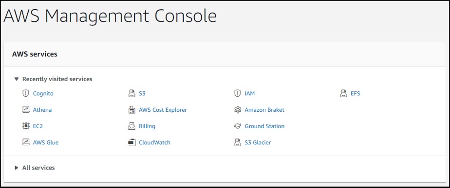
NOTE: If you are logged out or get kicked out of the console, simply return to https://codeathon.ncbi.nlm.nih.gov and log in again (remember your newly created password!) to get back to the console home page.
NOTE: This login method is unique to the workshop. If you want to create your own account after the workshop, visit the link below and follow the steps: https://aws.amazon.com/premiumsupport/knowledge-center/create-and-activate-aws-account/
Before we can use Athena, we need to make an S3 bucket that we can save our results to as we search the SRA metadata tables. So, let’s go make one!
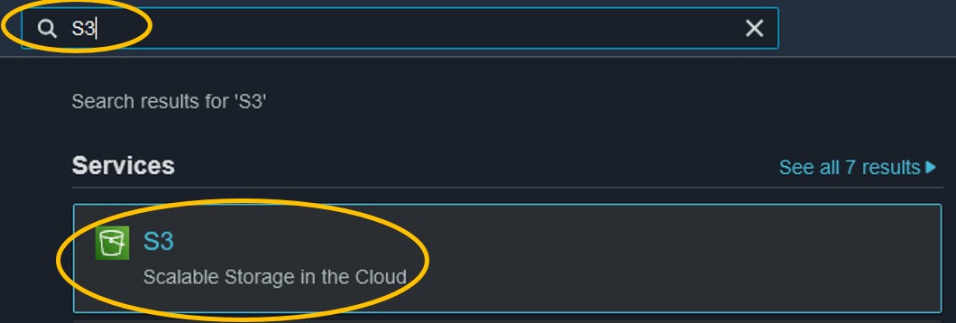
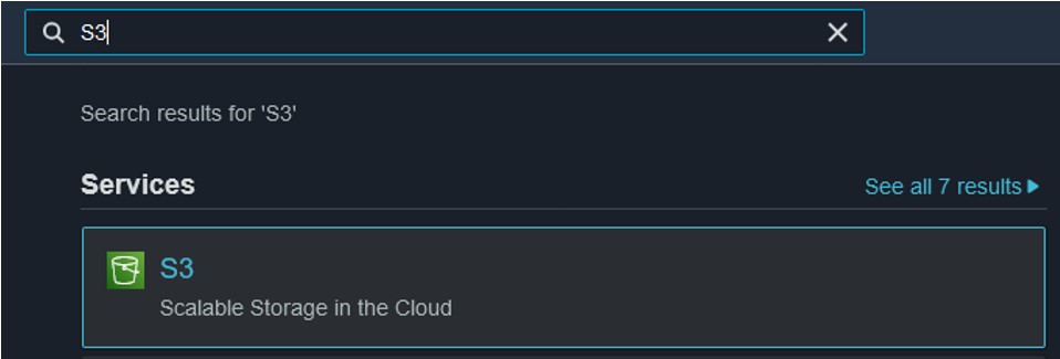
1) Use the search bar at the top of the console page to search for S3 and click on the first result
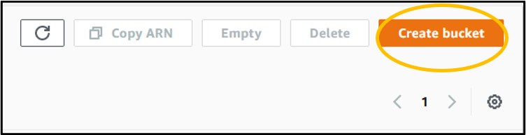
2) Click the orange Create Bucket button on the right-hand side of the screen
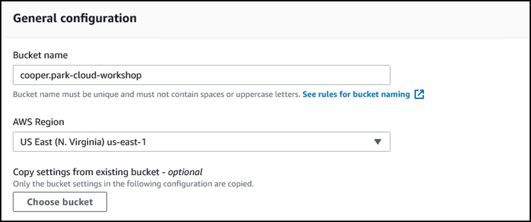
3) Enter a bucket name and make sure the region is set to US East (N. Virginia) us-east-1
S3 bucket names must be completely unique.
For this workshop, use the format <username>-cloud-workshop where <username> is the username you used to login
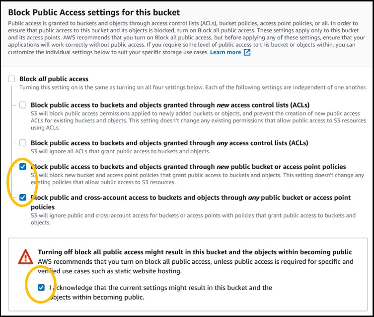
4) Scroll down to the Block Public Access settings for this bucket section. Deselect the blue checkbox at the top and select the bottom 2 checkboxes. Then check the box underneath the warning symbol to acknowledge your changes to the public access settings
NOTE: We turn on Public Access so that we can upload our files from the bucket directly to public websites like NCBI (e.g., we will be uploading result files from our bucket to the Genome Data Viewer later today). By default, you should keep your bucket from Public Access unless you explicitly need it
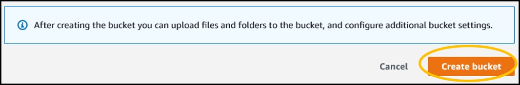
5) Ignore the rest of the settings and scroll to the bottom of the page. Click the orange Create Bucket button.
6) Clicking the button will redirect you back to the main S3 page. You should be able to find your new bucket in the list. If so, you have successfully created an S3 bucket!

Now that we have an S3 bucket ready, we can go see what the Athena page looks like!
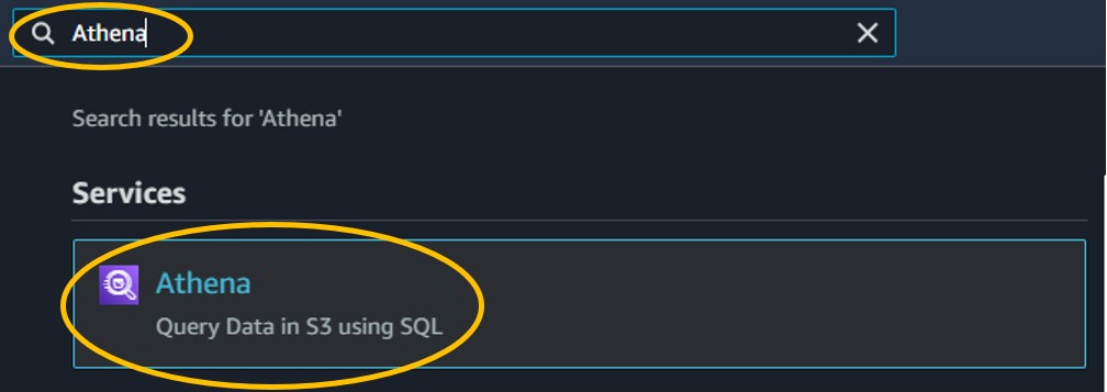
1) Use the search bar at the top of the console page to search for Athena and click on the first result
2) Visiting the Athena page should prompt you with one notification about the “new Athena console experience”. You can just click the “X” to remove it.
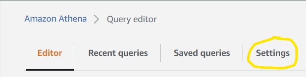
3) To make sure Athena saves our search results in the correct S3 bucket, we need to tell it which one to use. Good thing we just made one, eh? Click Settings in the top left of the screen
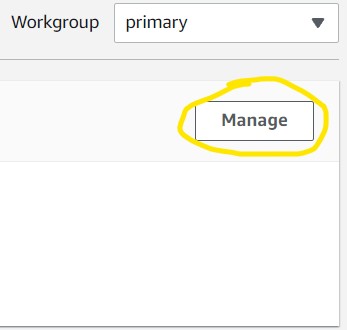
4) Click the Manage button on the right (1st image) then Browse S3 on the next page (2nd image) to see the list of S3 buckets in our account. Scroll to find your S3 bucket then click the radio button to the left of the name and click Choose in the bottom right (3rd image). Finally, click Save (4th image).

Now that we can save Athena results we can run some searches! The very last step to doing that is to import the table we want to search into Athena using another AWS service - Glue. However, to save time, this has already been done prior to the workshop by the instructor.
For the detailed instructions on using AWS Glue to add a table to Athena, visit the Supplementary Text: Instructions for AWS Glue!
These steps aren’t necessary to do before every Athena query, but they are useful when exploring a new table.
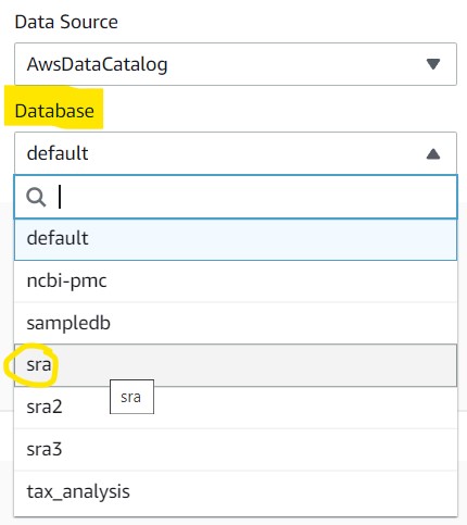
1) Navigate back to the Editor tab and click the dropdown menu underneath the Database section and click sra to set it as the active database. If you do not see this as an option, refresh the page and check again.
2) Look at the Tables section and click the ellipses next to the metadata table, then click Preview Table to automatically run a sample command which will give you 10 random lines from the table
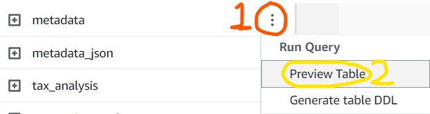
You can also click the + button next to the Metadata name to see a list of all the columns in the table.
For SRA based tables, you can also visit the following link to get the definition of each column in the table: https://www.ncbi.nlm.nih.gov/sra/docs/sra-cloud-based-examples/
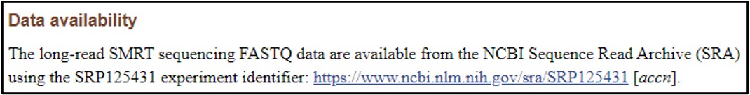
1) The following link is the actual publication for our case study today. Scroll to the very bottom and find the Data Availability section: https://www.ncbi.nlm.nih.gov/pmc/articles/PMC5778042/
You can also use the SRA Run Selector on the NCBI website to download data from NCBI directly to your S3 bucket! Find more information and a tutorial here:
https://www.ncbi.nlm.nih.gov/sra/docs/data-delivery/
2) The paper stored the data we need under and ID SRP125431, but we don’t know exactly which column that is associated with. So, scroll through the preview table we made earlier to find a column filled with similar values.
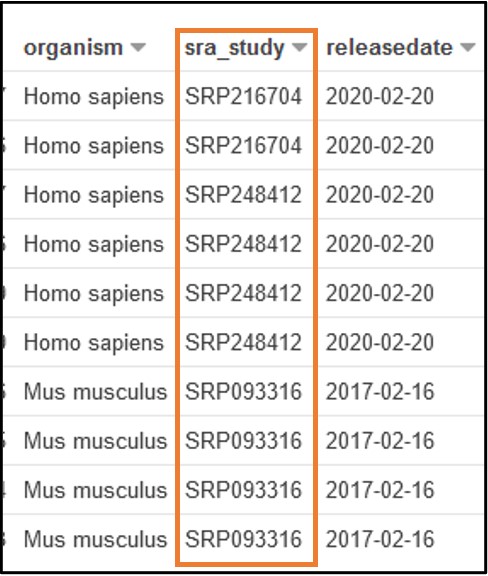
The Preview Table query we used to make this example pulls random lines from the table, so the values within your table may look different from this screenshot. The important info for us is that each value in this sra_study column starts with “SRP” (or “ERP”)
3) Now that we know which column to query for our data (sra_study), we can build the Athena query. Look to the panel where we enter our Athena queries. Click New Query 1 to navigate back to the empty panel so we can write our own query.
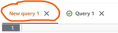
Fun fact: If you navigate back to Query 1 you should still see the result table for that query! Athena will save that view for you until you run a new query in that tab or close the webpage.
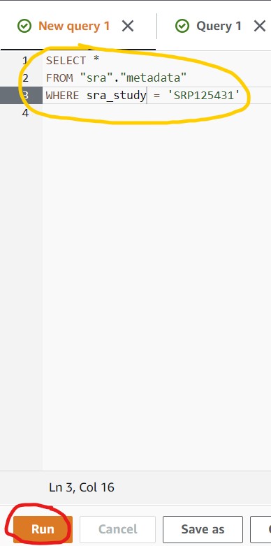
4) Copy/paste the following command into the query box in Athena (circled in yellow), then click the blue Run Query button (circled in red).
SELECT *
FROM "sra"."metadata"
WHERE sra_study = 'SRP125431'
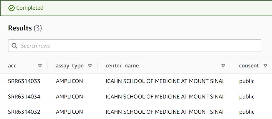
5) If you see a results table with three rows like the partial screenshot below, you have successfully found your data!
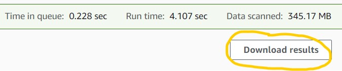
6) Click the Download results button on the top-right corner of the results panel to download your file to your computer in CSV format. You should be able to open this in Microsoft Excel, Google Sheets, or a regular text editor (e.g., Notepad for PC, TextEdit for Mac). We will review this file later, so keep it handy.
Want to challenge yourself? Visit the supplementary text (section: SQL challenges) to find some questions you can build your own SQL query for. Plus, find more advanced SQL query techniques and a deeper breakdown of the SRA metadata table too!
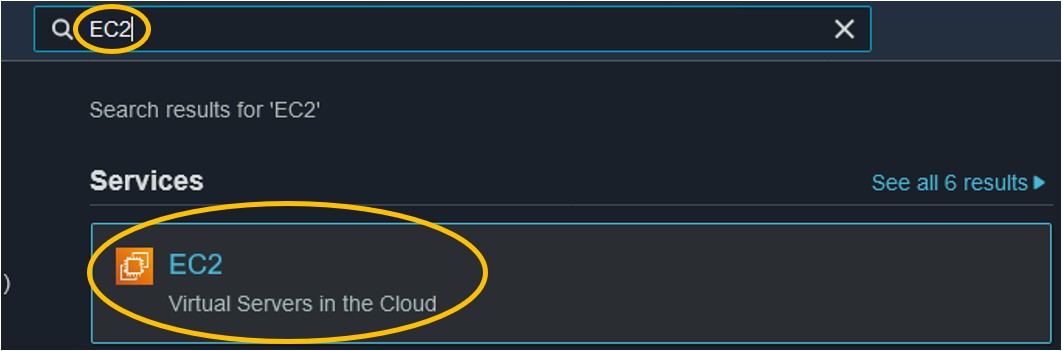
1) Use the search ar at the top of the console page to search for EC2 and click on the first result
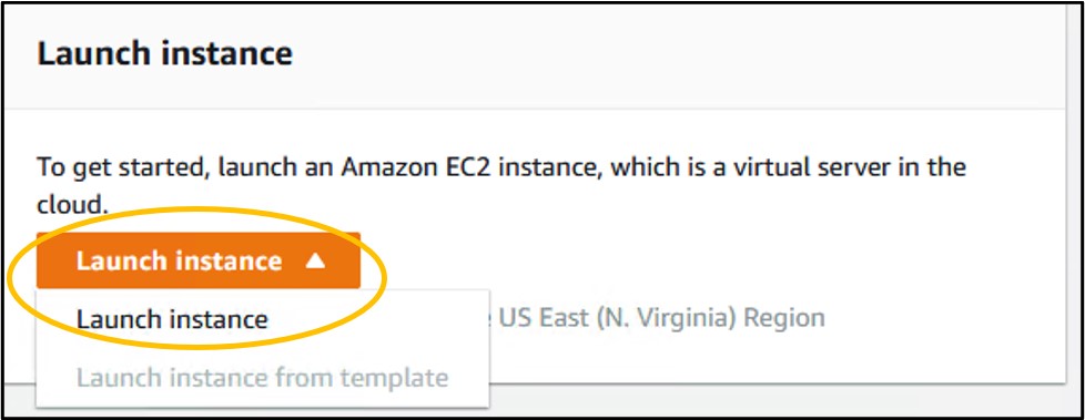
2) Scroll down a little and click the orange Launch Instance button and Launch Instance from its drop-down menu
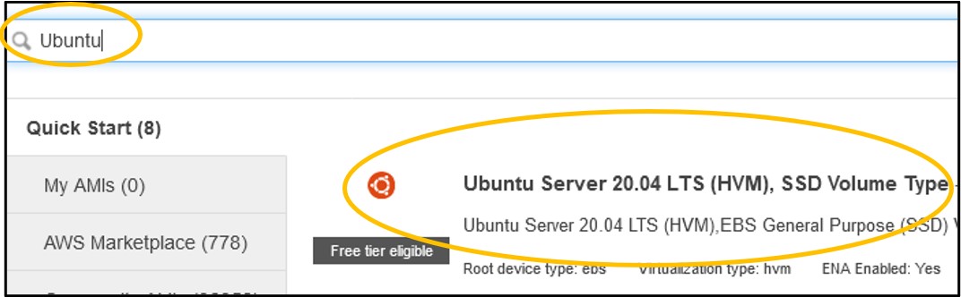
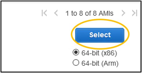
3) On the Step 1: Choose an Amazon Machine Image (AMI) page - type Ubuntu into the search bar and hit enter (top image) then click the blue Select on the right hand-side of the Ubuntu Server 20.04 image option (bottom image).
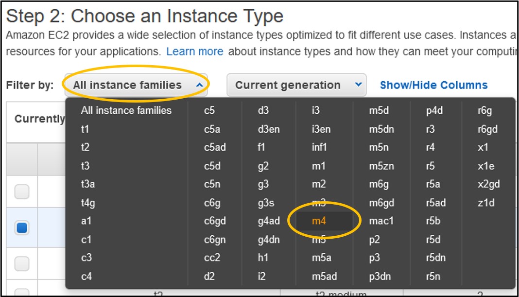
4) On the Step 2: Choose an Instance Type page - use the filter menus near the top of the menu to set the Instance Family to m4
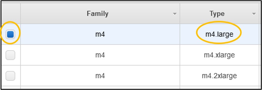
5) Look to the table below the filter buttons and check the box in the 2nd row from the top where the type is m4.large
6) Click Next: Configure Instance Details

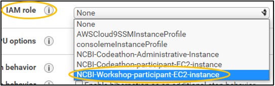
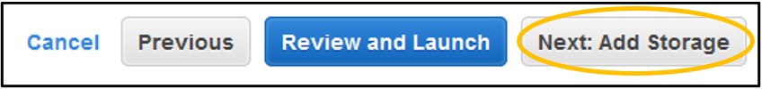
7) On page Step 3: Configure Instance Details - set the IAM role to NCBI-Workshop-participant-EC2-instance (top image). Leave all other settings alone and click Next: Add Storage in the bottom right (bottom image)
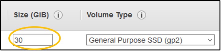
8) On page Step 4: Add Storage - Change the Size (GiB) to 30 (top image), then click Next: Add Tags in the bottom right (bottom image)
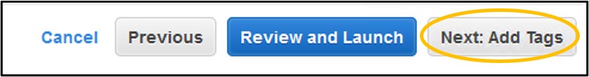
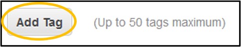
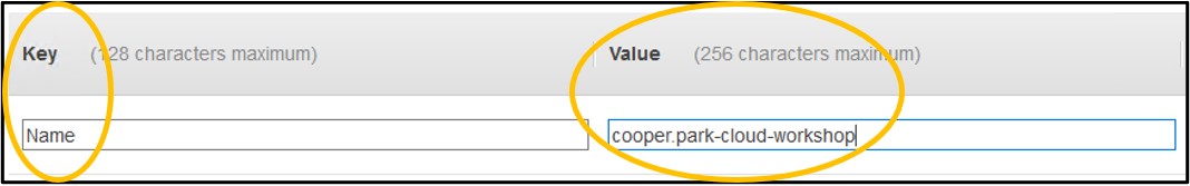
9) On page Step 5: Add Tags - Click Add Tag on the left side of the screen (top image). In the new row set the Key to be Name and the Value to be <username>-cloud-workshop just like we did with the S3 bucket earlier (bottom image). Remember, <username> is the username you logged into the console with.
10) Click Next: Configure Security Group in the bottom right of the screen

11) On page Step 6: Configure Security Group - Near the top of the screen, click Select an existing security group. Then click the box of the Default row at the top.
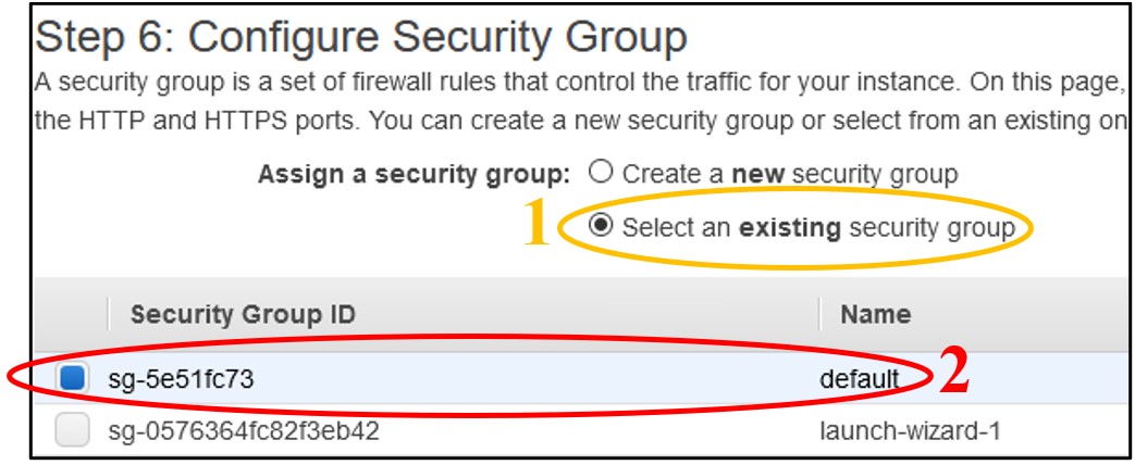
NOTE: This “default” network setting configuration leaves the instance open to public access. Typically you will want to restrict this to only trusted IP addresses, but for the purposes of the workshop we keep this open so there is no need to troubleshoot network issues. To balance this security flaw, we will restrict access to our instances with another instance feature in a few more steps.
12) Click Review and Launch in the bottom right of the screen

13) On page Step 7: Review and Launch – You should see two warnings at the top of the screen denoted by the symbol below. You can disregard these.
NOTE: The first warning tells us that our instance configuration will cost us money. The second warning tells us that our network settings make our instance publicly accessible, which is discussed in the above “NOTE”.
14) Click Launch in the bottom right of the screen.

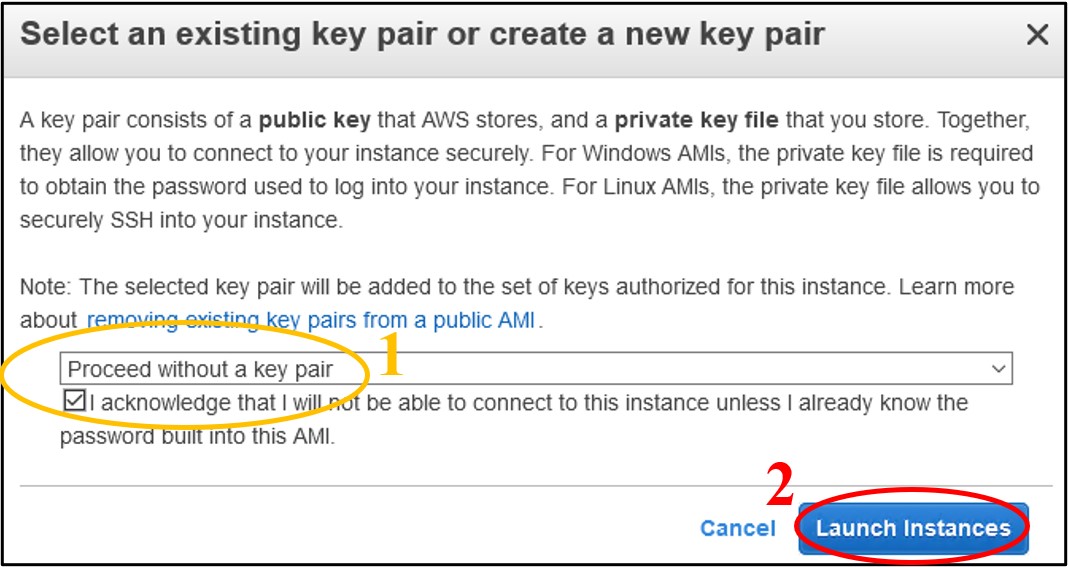
15) On the pop-up menu – change the first dropdown menu to Proceed without a key pair and check the box below it to acknowledge the change. Finally, click Launch Instances in the bottom right of the popup.
NOTE: Key pairs are used to access this remote computer using other methods, like SSH. We won’t be using these other methods so we can skip the key pairs here without affecting our ability to do the workshop. Additionally, by disabling the key pairs we also prevent public access to the instance. (This is how we will secure our instances for the workshop)
16) On the Launch Status page – Click View Instances in the bottom right
17) On the Instances page – Find your instance in the table of created instances and look to the Status Check column to see the status of yours.

18) Refresh the page occasionally until the Status Check column changes to 2/2 checks passed for your instance. This means we can now log into the instance.
NOTE: There are several ‘statuses’ this column can have. 2/2 checks passed is the final status. So, if you see anything else in the Status Check column, the instance is not ready to go.

19) Check the box to the left of your instance name (top image) to select the instance, then click Connect in the top right to head to the instance launcher (bottom image)

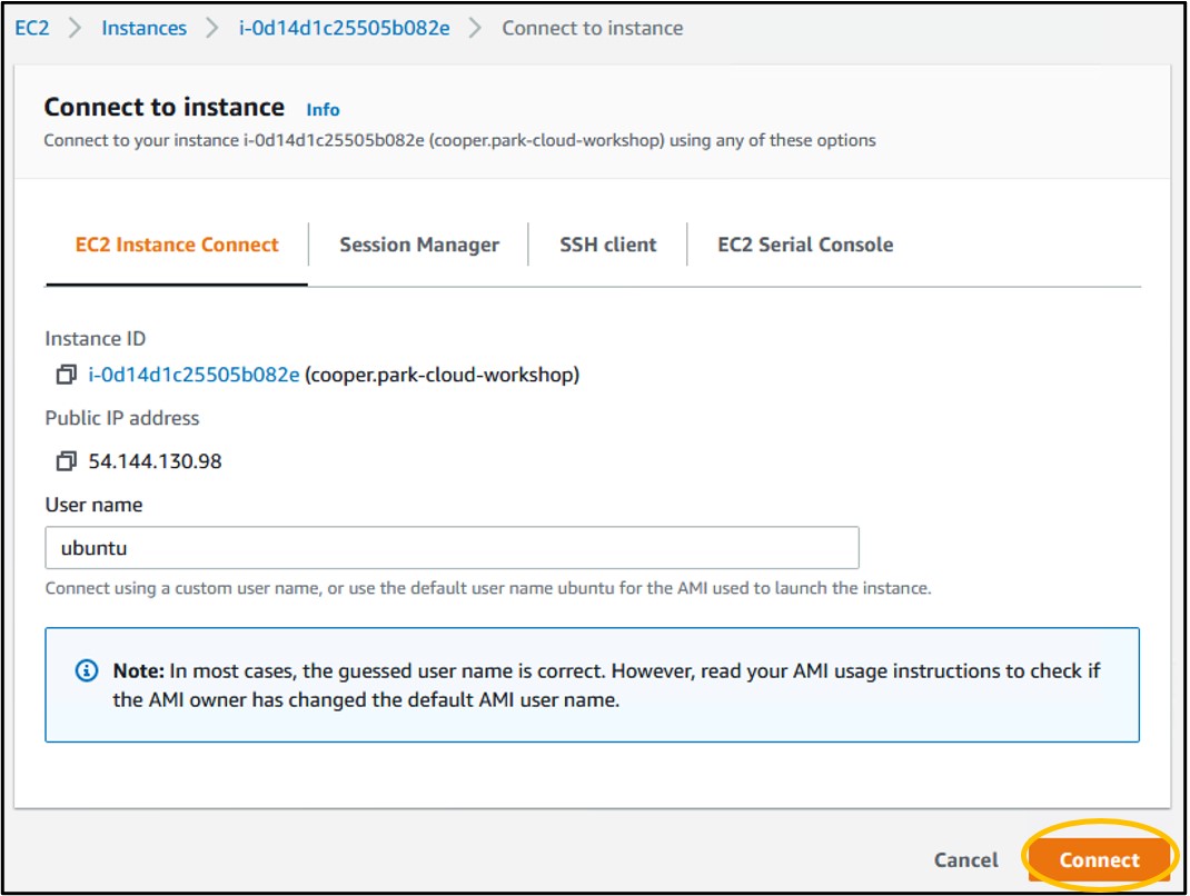
20) On the launcher page, click Connect in the bottom right. This will launch a new tab in your browser and connect you to your remote computer!
Before we can do our analyses, we need to install some software into our new remote computer
1) First we need to update the pre-installed software in our terminal. Copy/paste the following command into your terminal, then hit Enter
sudo apt-get update
2) To download magicBLAST, copy/paste the following command into your terminal, then hit Enter
curl -o magicblast.tar.gz https://ftp.ncbi.nlm.nih.gov/blast/executables/magicblast/LATEST/ncbi-magicblast-1.6.0-x64-linux.tar.gz
3) We also need to unpack the software so we can run it. Run the following command to do that
tar -xvzf magicblast.tar.gz && chmod -R 755 ncbi-magicblast-1.6.0/
4) Next, we need to install samtools. Run the following command below to do that.
sudo apt install -y samtools
5) Finally, we need to install the AWS command line interface. Run the following commands to do that
sudo apt install -y unzip
curl -o awscliv2.zip https://awscli.amazonaws.com/awscli-exe-linux-x86_64.zip
unzip awscliv2.zip
sudo ./aws/install
We can (finally) run MagicBLAST to align some reads! We just need two pieces of information to run the program.
A. The reference sequence – Will be solved with Step 1 below
B. The accession numbers for our reads – Will be solved with Step 2 below
1) Based on the information from the manuscript, we know that the deleted region in the genome is on Chromosome 7. In NCBI, the accession number for this sequence is NC_000007 so we can download this sequence to our remote computer and use it as the reference sequence for our alignment. Download the sequence using the following command.
curl -o chr7.fa 'https://eutils.ncbi.nlm.nih.gov/entrez/eutils/efetch.fcgi?db=nuccore&id=NC_000007&rettype=fasta'
2) Our Athena query gave us three different accession numbers that could be the child’s sequence data. To find out which one is associated with the child, scroll through the columns to find one that distinguishes each accession (hint: it’s the library_name column).
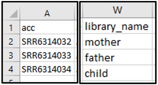
3) It looks like SRR6314034 is the ID we want! To run MagicBLAST on our selected accession ID, run the following command. This should take ~1 minute to run. You’ll know it worked okay if the command runs with NO output.
./ncbi-magicblast-1.6.0/bin/magicblast -subject chr7.fa -sra SRR6314034 -out SRR6314034.sam
4) Next, we need to format the output files so that we can use them in Genome Data Viewer. Run the following samtools commands to do this. it will run each samtools command in order automatically. Like above, if NOTHING happened after hitting enter, then it worked!
samtools view -S -b SRR6314034.sam > SRR6314034.bam
samtools sort SRR6314034.bam -o SRR6314034.sorted.bam
samtools index SRR6314034.sorted.bam SRR6314034.sorted.bam.bai
5) Now we’ll move all these results files to a single folder so we can keep track of them
mkdir results && mv SRR* results/
6) Finally, we need to move these results files to our S3 bucket so we can access them outside of our AWS account. Run the following AWS CLI command to copy the files to your S3 bucket.
REMEMBER: You will need to replace the
<username>piece of the command with your own login username to make it match your S3 bucket name. So copy/paste the command into your terminal, then use the arrow keys to move your cursor back through the string and change the name to your own bucket.
aws s3 sync results/ s3://<username>-cloud-workshop
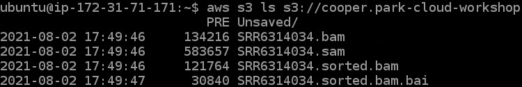
7) To check if we got all of our files moved to our s3 bucket we can run one final command (remember to change the <username> portion again here):
aws s3 ls s3://<username>-cloud-workshop
8) We should now be done with our remote computer (aka: EC2 instance). Go ahead and close the browser tab your instance is open in.
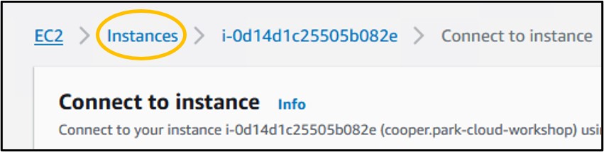
9) In the console webpage, click the blue Instances button at the top of the instance launcher page
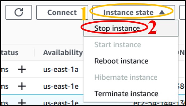
10) We don’t want to leave an instance on while not using it, because it costs money to keep it active. So, let’s shut it down, but not delete it, just in case we want to use it later. Check the box next to your instance (top image) then click the Instance State drop-down menu and select Stop Instance (bottom image).

11) Finally, we need to check on the files in our S3 bucket and make them publicly available to upload the files to GDV later. Navigate back to the S3 page (use the search bar at the top of the console page) (top image) and click on your bucket name (bottom image) to see its contents
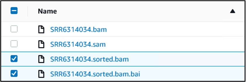
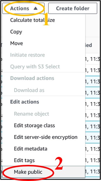
12) You should have four files in your bucket. We need the files that end in sorted.bam and sorted.bam.bai. Check the box next to each of those files (top image) then use the Actions drop-down menu and select Make Public at the very bottom (bottom image)
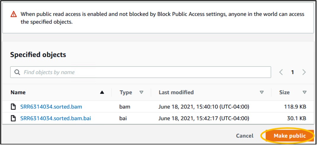
13) On the new page, click the orange Make Public button in the bottom right of the page to make the files publicly accessible
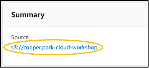
14) If it works, you will see a green banner at the top of the new page like seen below (top image). If you see this, click your bucket link under the “summary” panel (bottom image) to navigate back to the main bucket page.

1) Open a new tab in your web browser and go to https://ncbi.nlm.nih.gov/genome/gdv/
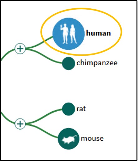
2) Make sure the Human is selected from the tree on the left
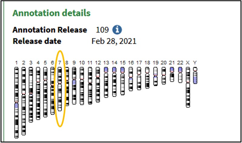
3) Scroll to the bottom of the page and click on the 7th Chromosome image to load the Genome Data Viewer on the human reference genome’s 7th chromosome
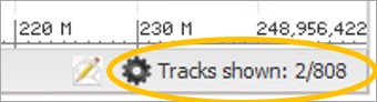
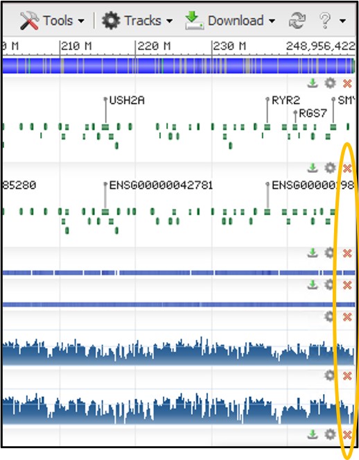
4) The GDV page comes pre-loaded with several tracks aligned against the chromosome. Most of these are not useful to us today, so we can use the red X buttons in the top right corner of each track to delete them. Do this for every track except the top one. This top track shows every gene and its position on the chromosome.
There are LOTS of NCBI-offered tracks you can upload ato compare against your own data. To learn more about them click the little gear at the bottom of the viewer page:
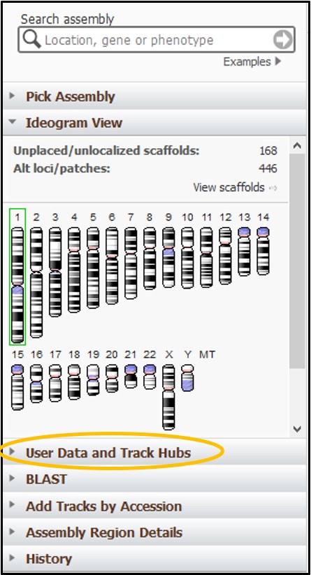
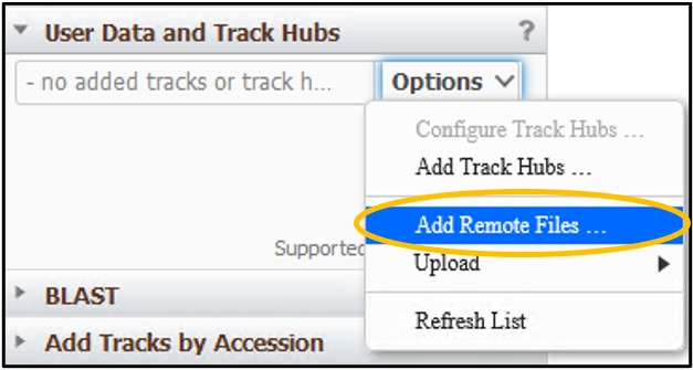
5) Now we can add our own tracks to the viewer. Click on User Data and Track Hubs on the left side of the screen
6) Click the Options pulldown menu and click Add Remote Files…
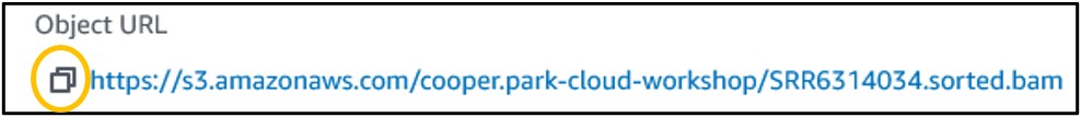
7) Navigate back to your S3 bucket tab and click on the SRR6314034.sorted.bam file to open up the details for the file

8) On the new page, click the “Copy” button next to the Object URL to copy the URL path to the file to your clipboard
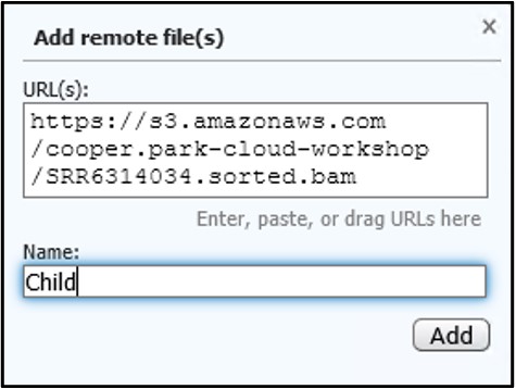
9) Go back to your GDV tab and paste the link into the URL box. Next, add a familiar name like Child to the Name box to help us identify the track later. Then click Add
10) This track is showing all of the results of magicBLAST in a “pile-up” view. This is basically one long histogram plot where a taller bar represents a region of the chromosome where more reads from the sample aligned to. Because our sequences are specific to a single gene in the chromosome, but our current view is showing the entire chromosome, the pile-up view may look a little bland.
Try to find the region of the chromosome that our reads aligned to:
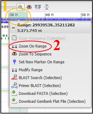
11) Use the scale bar at the top of the viewer and click-and-drag across the section where our reads aligned to highlight it. Then use the pop-up menu to click Zoom On Range
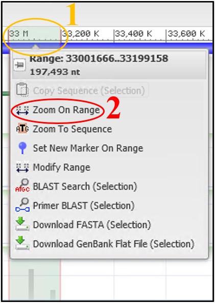
12) Repeat step 14 using the new view to refine the range again if the view didn’t change very much.
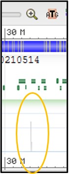
13) Your view should now see the track similar to the screenshot below. If you don’t see the mess of red lines below the thick black bar, that’s okay! We will turn it off next anyway.
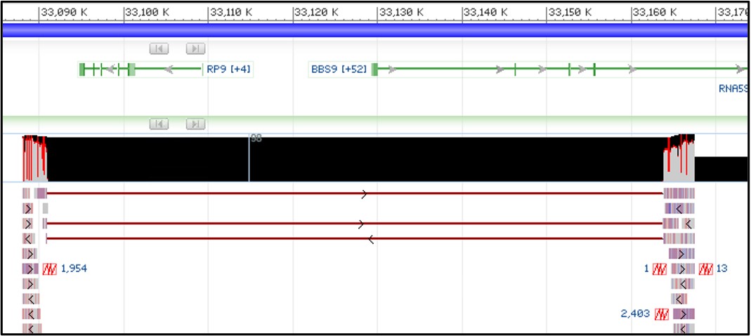
NOTE: The tracks may be slightly different depending on how you have zoomed in. As long as you can see the image above somewhere on your screen you are doing great!
14) Those red lines underneath the thick black box are showing how each individual sequence read aligned to the reference sequence. This particular view isn’t very helpful to us, so let’s turn it off.
NOTE: If you can’t see these lines, that’s great! You can skip Steps 15 & 16
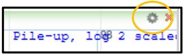
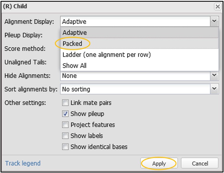
15) Click the little gear in the top right corner of our Child track to open its settings.
16) On this new menu page, change the “Alignment Display” to “Packed” and then click Accept. You can change many other settings here as well, but I’ll leave that up to you to explore outside of this workshop.
Now that we can see the range a bit better, let’s break down what each of these colors represent in the pile-up view:
If you want to explore the pile-up view a bit more, try using the buttons in the toolbar just above the numeric range to navigate the assembly. Hold your mouse over the button for a description of what they can do!
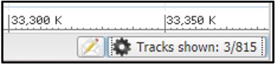
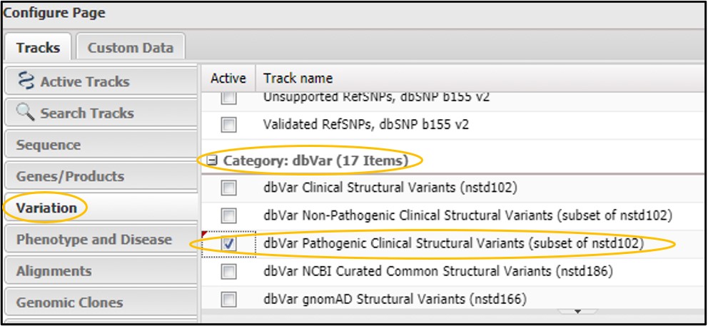
1) Click the Tracks button in the bottom right corner of the viewer panel to open the Configure Page
2) Click on the Variation tab and scroll way WAY down to the dbVar category. Then click the checkbox next to dbVar Pathogenic Clinical Structural Variants then click Configure in the bottom right corner of the page.
3) You should now have a new structural variants track loaded into the viewer. This track shows the region of the genome where each variant is found. Blue variants are caused by an insertion in this region, while Red variants are caused by a deletion. Because our alignment suggests a deletion, we want to focus on the red variants.
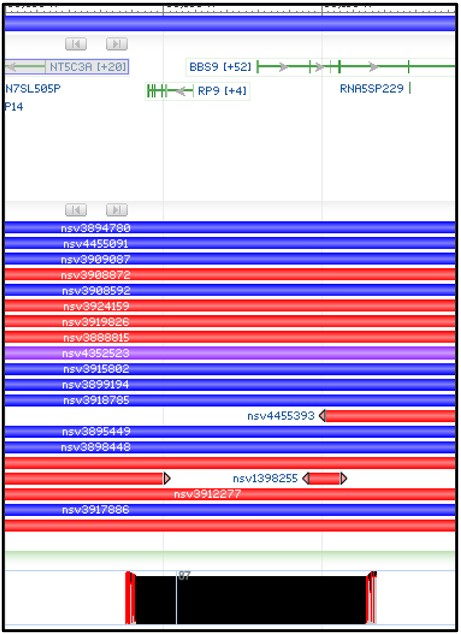
4) Next, zoom in on the right-half of our aligned region in the child track like the screenshot below. We want to look closely at the BBS9 gene to find structural variants that overlap with this region.
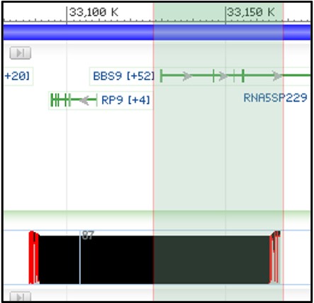
5) Obviously, there are a LOT of variants that overlap in this region. However, our concern is only about our sequenced region of the gene. Variants which extend beyond our sequenced region are less likely to be relevant for us. So rather than just aimlessly checking every red variant, lets look only for variants that start or stop within our deletion.
Oh… there’s just one? Let’s check that one then.
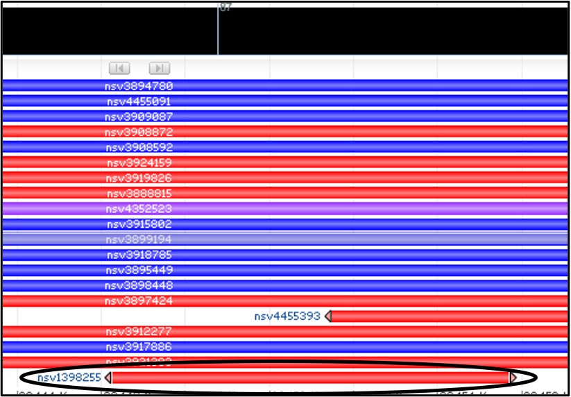
6) Mouse over the variant nsv1398255 to get a new pop-up menu and select the dbVar link at the bottom of it
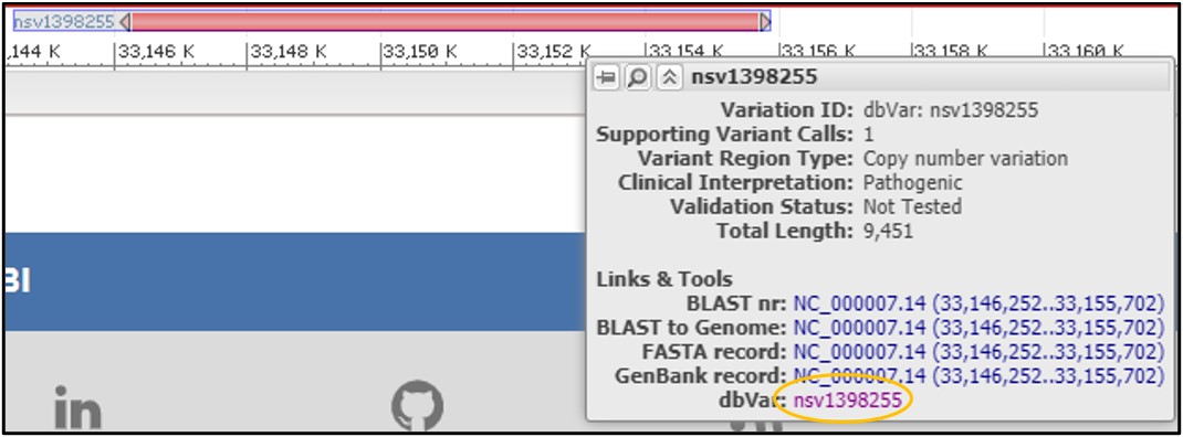
7) On the dbVar page, navigate to the Clinical Assertions panel to see which clinical conditions have been associated with this deletion
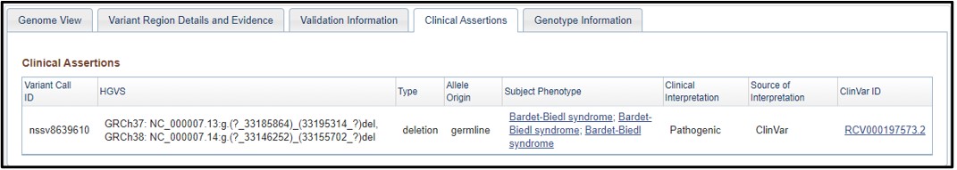
8) Just as we suspected! This region is associated with Bardet-biedl syndrome. If we wanted to, we could click on the phenotype and explore more about the condition. But that is something you need to explore on your own, because this is the end of the worksheet!
This concludes our exercise on navigating the AWS Cloud computing console and several of its most popular cloud services. We hope that you are motivated to take these skills and tools with you and explore how they can benefit your own research. You can find links to many useful resources to help you below.
AWS
Genome Data Viewer
MagicBLAST
SRA
In order search through a table (like the SRA metadata table) you need to load it into Athena. Because this is your first-time accessing Athena, it shouldn’t be a surprise that you don’t currently have any data tables loaded! Therefore, our first step will be to add the SRA metadata table to Athena. There are three ways you can add a table to Athena:
Create the table using SQL commands (we are not SQL experts here…yet, so we won’t do it this way)
Add the table manually from an S3 bucket (although the SRA metadata is stored in its own S3 bucket, we don’t know the format of the table, so we can’t do it this way)
Use another AWS service called AWS Glue to automatically parse a table and load it into Athena for us using a “Crawler” (this is what we will do)
Note: Although AWS Glue is the most convenient method, it is also the only one to cost money. To parse the SRA metadata table it will be… ~$0.01.
This section will walk through the steps taken during the AWS Glue demo to prepare the SRA metadata table for Athena queries
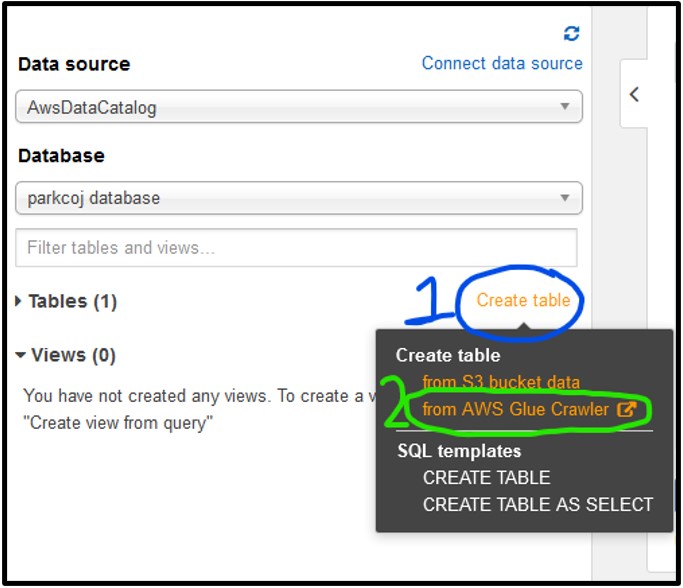
1) To start working with AWS Glue, navigate to the Tables section of the Athena page on the left-hand side, then click Create Table and select from AWS Glue Crawler as seen below. If you see a pop-up about the crawler, just click Continue.
2) The settings for this crawler should e set as described below:
Next page
Next page
Next page
Next page
Next page
Next page
Next Page
Click Finish
3) You should now be on the Crawler page for AWS Glue. Here you can manage and run crawlers. Click the checkbox next to the new crawler and select Run Crawler
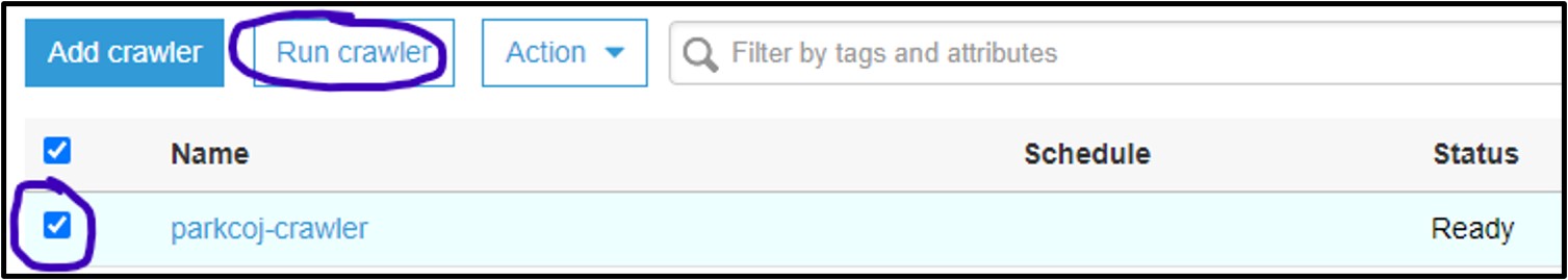
4) If it worked, you should see the Status column say Ready again, and the Tables added column should have changed to 1:

5) The table should now appear in Athena and you can follow the same steps described in section Exploring Athena Tables above.
Now that you have a handle on how SQL commands work, let’s try some examples! Remember, you can use the “Tables” section on the left-hand side of the page to find out which columns you can filter by in your table.
If you find yourself stumped on the answer to any of these, or just want to check your answer, click the dropdown box underneath the question to reveal the solution and see a screenshot of the results table!
a) You just came across a new paper with lots of great sequence data. You want to add that data to your own research so you jump to the paper’s Data Availability section (because all great computational papers have one!) and see that the data was stored in an SRA study under the accession SRP291000. Write a SQL command in the query terminal to find all data associated with the SRA study accession SRP291000:
SELECT * FROM "sra"."metadata" WHERE sra_study = 'SRP291000'
b) You are working on a new genome assembly tool for short-read sequences. However, you don’t have any reads of your own to test it! You know that SRA metadata includes the sequencing platform reads were generated on, so you decide you want to check there. Write a SQL command in the query terminal to find all data sequenced with the OXFORD_NANOPORE platform.
SELECT * FROM "sra"."metadata" WHERE platform = 'OXFORD_NANOPORE'
Now let’s get a little bit more complicated with our queries by combining multiple filtering conditions together. For example, see the command below:
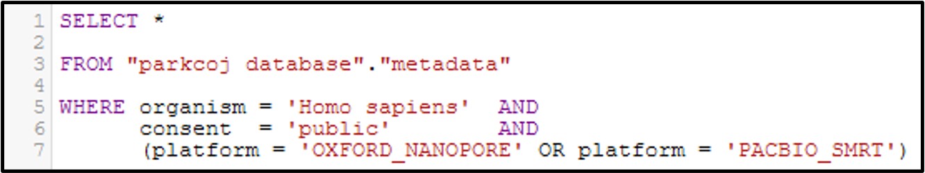
In this command we use the AND statement to add multiple requirements for our data. Specifically, we added a second criteria where the consent = public (aka: The data is not under restricted access). Additionally, we add a more complex requirement by using an OR statement for the platform column to ask for data that was generated by the OXFORD_NANOPORE OR PACBIO_SMRT sequencing platforms. Overall, by running this command we will only get the data that fits all 3 conditions.
Note: Make sure you include parenthesis around an OR statement as seen above, otherwise the query may not work as intended.
Here’s a few brain teasers to flex your new SQL skills! Remember, if you are stuck you can click the dropdown box underneath the question to reveal the solution and see a screenshot of the results table!
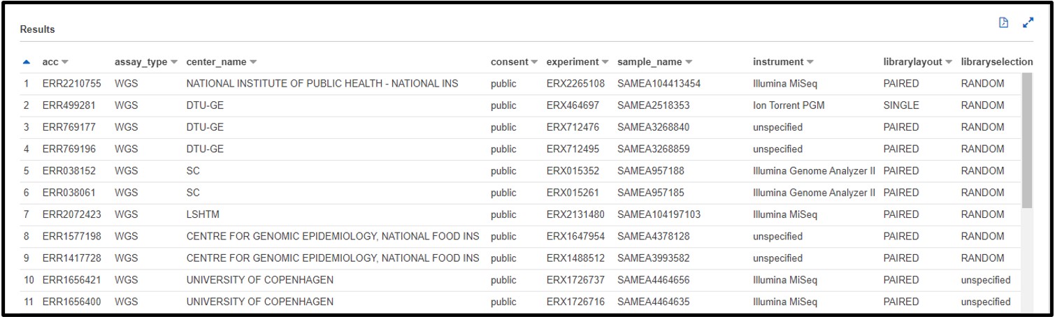
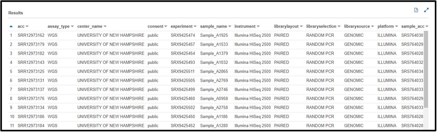
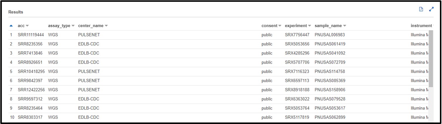
a) After testing your genome assembly tool from earlier, you realize that not all Illumina datasets are created equally! It turns out you only need WGS (Whole Genome Sequencing) genomic data to properly validate your software. Also, you noticed that there was some metagenomic and transcriptomic data mixed in with your test cases. So, this time you are just going to look for “genomic” datasets. Write a SQL command in the query terminal to find all WGS assay_type data sequenced on the ILLUMINA platform and a GENOMIC library_source.
SELECT * FROM "sra"."metadata" WHERE platform = 'ILLUMINA' AND assay_type = 'WGS' AND librarysource = 'GENOMIC'
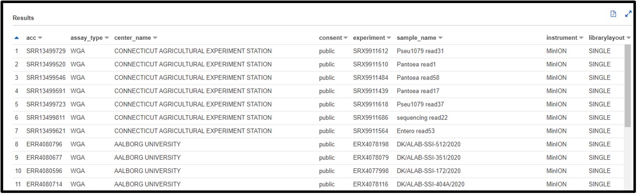
b) You are designing a population-level epidemiological survey of some bacterial pathogens from samples collected across Europe. You decide you want to get some preliminary data on Escherichia coli (or maybe Staphylococcus aureus…) from the SRA, but you aren’t picky about what kind of sequencing is done just yet. Write a SQL command in the query terminal to find all sequences collected from the continent Europe and are from the organism Escherichia coli or Staphylococcus aureus.
Hint: The column header for the continent is not very intuitive. Try using the “Preview Table” option from the “Tables” tab described earlier to find a column that would fit.
SELECT * FROM "sra"."metadata" WHERE (organism = 'Escherichia coli' OR organism = 'Staphylococcus aureus') AND geo_loc_name_country_continent_calc = 'Europe'